ANN Modeling to Predict the COD and Efficiency of Waste Pollutant Removal from Municipal Wastewater Treatment Plants
Saeed Pakrou1 * , Naser Mehrdadi2 and Akbar Baghvand3
1
Civil Engineering – Environmental,
Aras International Campus,
Iran
2
Civil Engineering – Environmental,
University of Tehran,
Iran
3
Civil Engineering, Environmental,
University of Tehran,
Iran
http://dx.doi.org/10.12944/CWE.10.Special-Issue1.106
The system in this study is modeled by neural network and studies conducted in simulating the presumptive developed sewage treatment plant with the single activated sludge process and SSSP software along with the system’s experiences. The results obtained by the developed neural network model are analyzed for the presumptive treatment plant. The maximum correlation coefficient is 0.98 for modeling the presumptive waste treatment plant. Using real data from the Tabriz waste treatment plant, the best and most appropriate neural network model is obtained as R equals to 0.898, the maximum removal efficiency of the treatment plant relating to the TSS pollutant is equal to 94 percent, and the minimum removal efficiency related to TS is equal to 38 percent. Likewise, the removal efficiency of mentioned pollutants is equal to 95 and 37 percent estimated by the neural network, respectively, which indicates a relatively high accuracy considering the error percentage existing in the input data.
Copy the following to cite this article:
Pakrou S, Mehrdadi N, Baghvand A. ANN Modeling to Predict the COD and Efficiency of Waste Pollutant Removal from Municipal Wastewater Treatment Plants. Special Issue of Curr World Environ 2015;10(Special Issue May 2015). DOI:http://dx.doi.org/10.12944/CWE.10.Special-Issue1.106
Copy the following to cite this URL:
Pakrou S, Mehrdadi N, Baghvand A. ANN Modeling to Predict the COD and Efficiency of Waste Pollutant Removal from Municipal Wastewater Treatment Plants. Special Issue of Curr World Environ 2015;10(Special Issue May 2015).
Available from: http://cwejournal.org?p=702/
Download article (pdf)
Citation Manager
Publish History
Introduction
Protecting water resources as the most vital substance for human need has been considered increasingly by different international assemblies. Population growth, which leads to excessive utilization of scarce water resources on one hand, and their contamination due to a variety of biological, agriculture and industrial activities of mankind on the other hand have activated the alarm of water crisis in the years to come. Therefore, preserving the physical, chemical and biological quality of water resources is the frontispiece of many organizations that somehow deal with these resources. (Mogens Henze, 2007).
Active sludge, which is an aerobic suspended growth treatment system, developed by Ardern and Lockett in 1914, and became very popular at the same time, because its process included producing activated microorganisms which were able to be activated aerobically. Many versions of this process are being used everywhere by considering the fact that their bases are similar (Tchobanglous and Burton, 1991).
Intelligent visualization and error detection to achieve the optimum performance in wastewater treatment plants using the Artificial Neural Network (ANN) detection technique has a very active research area in recent years. Artificial Neural Network, as one of the modern modeling techniques, has been under special consideration more recently. These models are applicable for prediction and classification in cases where statistical classical methods are not usable because of their limitations. Therefore, it is tried in this research to design the proper model for evaluating the performance of municipal wastewater treatment plant as well as identifying the effective factors in the performance of municipal treatment plants. Sensitivity analysis is being used in order to determine the sensitivity of a model to change in its parameters and also in its structure. Since the sensitivity analysis represents the model behavior along with the change in its parameters, it could be a useful tool for modeling and evaluating models.
There is usually a slight uncertainty in modeling to choose values which should be estimated (Forrester and Breierova and Choudhari, 2001).
Methods and Materials
The Tabriz wastewater treatment plant is built at a distance of four kilometers west of Tabriz in the Qaramalek village lands and on the south side of the Ajichay River in an area of 72 hectares with a capacity of 765000 M3/d wastewater which is being purified by the activated slug process. This wastewater treatment program has been planned for a population of six million by the year 2025.
Utilized Data
The Tabriz wastewater treatment plant was examined for 6 months (from June to November of the year 2013) regarding the COD removal. The assessment variables of the system included the temperature of the ambient air and wastewater, flow rate, pH, opacity, alkalinity, Suspended Solids (SS), COD, BOD5, the wastewater and sullage flows, and also various units in filtration education functions.
Neural Network Modeling
Back propagation Algorithm
Preprocessing
Preprocessing is a need for the weights of a neural network. Choosing the weight impact causes the network to reach a general mode or an area in reducing error or the way it converges. Normalizing the data is very important in the neural network. Hecht-Nielsen suggest to use two different sets of data during the training. One of these sets is being used for adjusting the weight and the other set is being used in time interval for calculating the error. The training is continuous if the error in the second training set continues to decline. The network starts to memorize the training patterns when the error in the training set starts to increase (named validation in the neural network toolbox of MATLAB). Consequently, the training section will stop (Konar, 1999).
The structure of the network has been defined before as the number of hidden neurons and hidden layers. The limitations on the number of neurons and hidden layers defined by Hecht-Nielsen (1987), and Roger and Dowla (1994) were selected as the basis for this research.
Coding and Matlab Neural Network Toolbox
Neural Network Toolbox and Gui
Developing this model is done with MATLAB version 2013 from MATH WORKS Company.
The neural network toolbox is mainly used in this research from a previously developed neural network using the written codes for automatically producing the artificial neural network in order to extract more accurate results.
Matlab Coding
A MATLAB code is written for developing the model, which automatically creates the artificial neural network for wastewater treatment plant. This code does the same thing as the artificial neural network GUI does.
Simulating The Treatment Processes
Simulation of Single-Sludge Process (SSSP) is chosen because it’s a very powerful simulator for the activated slug process such as nitrification and denitrification. In addition, one of the other reasons for choosing this simulator is its successful implementation in many simulating researches (Sin, 2000).
The treatment model consists of a chain of 1 to 9 reactors, which are totally mixed. Dynamic solution options in the SSSP software are being used to calculate a solution for mass balance equations in the intake concentration and flow, which alters in a cycle more than 24 hours. The SSSP software automatically calculates the average flow velocity and the average concentration of flow weight, and uses them to compare the start point for ordinary numerical integration. The computer then repeats this integration for more than a 24-hour cycle until the change in concentration stops from one cycle to another. In other words, the computer calculates the response of a system which receives the input 24-hour cycle every day (Bidstrup and Grady, 1987).
The accuracy of predicting is usually evaluated by providing data which are not introduced to the network before, and the ability of Root Mean Square Error (RMSE) is called generalization (R). In this regard, the correlation coefficient for validating designed networks, Mean Absolute Percentage Error (MAPE), and Mean Absolute Error (MAE) are used.
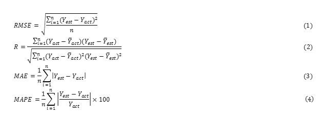
In which, n is the number of predictions; Yact is the real observed value; real observed value; Yest is the predicted value; Ȳact is the average of real observed value; and Ȳest is the average of predicted value extracted from the model (Mehdipour and Shokouhiyan, 2012).
Results
Activated sludge treatment unit, in this study, is modeled by the artificial neural network. One of the programs was presumptive developed sewage treatment plant using the SSSP simulator, first version, and the other one was the real program of treatment in Tabriz, Iran.
The presumptive wastewater treatment plant is built simply using the default parameters of SSSP and the default data of fine particles in the dynamic wastewater on behalf of the wastewater treatment plant, and the dependent variable values are achieved for the wastewater. In the following, the neural network model is created from a real wastewater treatment plant with the obtained data. The MATLAB code is written based on an automatic search process on the error surface with the aim of determining the minimum error in the trained model predictions.
The Studies of Treatment Process Simulating Model
Developing The Neural Network Models by the Data Program of Sssp Simulation
Developing of the neural network does at first by a hidden layer manually. The developed code for automatic model production is utilized after getting familiar with the neural network GUI toolbox. Two training functions are implemented according to the studies of the user manual for modeling (Trainbr and Trainb). The code was simple and it was working as follow:
The number of hidden neurons for each training function is changed from 2 to 10 (based on the algorithm). Thirteen training functions provided for implementing the back-propagation algorithm by the neural network MATLAB toolbox. Nine neural network models with different hidden neurons of 2 to 10 layers for each training function and consequently 117 models for each complete run of the code is developed.
The Guide Developing Neural Network Model Using the Toolbox Gui
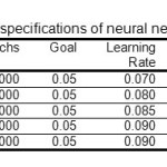
The manual performance showed that the model with 3 hidden neurons in the hidden layer has the least error and the best coordination with the main data. All other features of the neural network model are kept constant during the performance. Thereafter, the model with one hidden layer and 3 hidden neurons was chosen as the optimal model and the training rate changed in the training operations. The size of the epoch period has a significant decrease up to 6000, because the significant decrease in the mean square error is not noticeable after this point. Therefore, the performance stopped at the epoch period of 6000 (Table 1).
 |
|
The Data Studies of Neural Network Model in Tabriz Treatment Plant
Data Preparations of Tabriz Treatment Plant
Two different data sets are used for the neural network model of the Tabriz treatment plant. Eight variables were chosen from the system for building a neural network model in the modeling process. Different combinations of data are used in the process of model development. The system variables used in the modeling included solids retention time (ï±c), the flow rate of fine particles (Qinf), pH of fine particles, water temperature of fine particles (Tinf), concentration of fine COD particles, MLSS, sullage COD, wastewater TSS and the slug production rate of the primary sedimentation tank. These variables are used alone or combined with each other in order to predict the concentration of waste COD from the purified water of the treatment plant. Many combinations of the variables are used and hundreds of models are developed and trained to evaluate the effectiveness of prediction. Data preparation is done by eliminating the empty values from the main data set. The raw data has been established from about 6 months of daily measurements and 150 days for test at first, except Fridays, which consisted of about 450 data.
Preprocessing of the data from the Tabriz treatment plant is done by allocating the input and output data to the range [0, 1] or [-1, 1] after preparing them to develop the model. This transform is done for all the data points as follows:
For the interval [ 0, 1]:
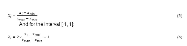
Each data variable should be fed into the neural network model using normalization of input data with nonlinear transfer functions such as logsig, tansig and with equal weight. Therefore, the data should be scaled by the equations (5) and (6) in the intervals [0, 1] and [-1, 1], respectively.
No good result is obtained in performing the interval [-1, 1]. In these runs, script was tested with one hidden layer at first. Then, the number of hidden neurons is changed based on the defined criteria by Hecht-Nielsen (1987). The maximum correlation coefficient achieves to 0.4 in these runs. The number of hidden layers, then raised to 2 layers. The logsig transform function is used for the interval [1, 0], and the tansig transform function is used for the interval [-1, 1], using the same data. There is the possibility of using the combinations of the transform function in multilayer models using a specific transform function in one layer and another transform function in a different layer. Some possible combinations in this function are as follows in the case of using two hidden layers (tansig-tansig, logsig-logsig, tansig-purelin, etc.).
Developing Ann for Tabriz Treatment Plant
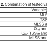
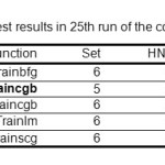
MATLAB software is used to create the neural network model automatically and using the data from the Tabriz treatment plant. Performing the script is started by determining a combination of variables being used together. Many variable combinations were used and it is tried to be continued when there was a good coordination between real data by visual judgment and considering the correlation coefficient, R, when there was an acceptable fitting. The best fitting was observed in the sullage COD data combined with MLSS, TSSeff, and Qinf in the combination 25 and the efficiency of R=0.898. Based on the observations, the specified variables in the combination 25 are used alone or as mates to create new subsets in the script and were tested in order to find the improved results. The combination of tested variable is provided in Table (2).
 |
|
The script automatically causes a change in the number of hidden neurons to improve the output in addition to the manuals of variable combination change. The output here was to predict the sullage COD. All these runs are performed for different hidden layers. On the first run, there was only one hidden layer and the number of hidden neurons changed from 1 to 9. As explained previously in the methods and materials section, there is 13 training function in the MATLAB toolbox of neural network for the base in the back-propagation algorithm. This script produces the neural network model using these continuous functions (Table 1). The tansig and logsig transfer functions are performed in different scripts. Then, the same method is used by the script for ANNs with two hidden layers. The number of hidden neurons in the next runs by script with two hidden layers also change from 1 to 9 for both hidden layers.
The best fitting of the neural network model is calculated regarding the highest correlation coefficient.
 |
|
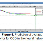
The mean square error is given for the best run in the training session in Fig. (4). The training session, at the period 48, stopped after the validation process finished. Three rules to stop the training session: 1) Achieving the goal, which reduces the mean square error to zero, 2) the number of failures gets higher from a specific amount, and 3) reach to the maximum number of given periods (2000 periods here). The stop criteria of 2 is used here at the best run to stop the training session. Different iterations based on the number of neurons in the hidden layer and the stimulus functions of hidden and output layers are provided in Table 3, for simulating the variations of qualitative parameter COD. All the models are in the training and evaluation stages.
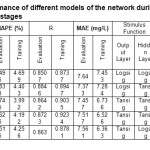 |
Table 3: Performance of different models of the network during the training and evaluation stages Click here to View table |
As it can be seen from Table (3), although the network training of Trial3 has resulted the best in the training stage, but the network training of Trial2 has provided better results in comparison with other trainings at the evaluation stage and have further generalizing power in respect to other trainings.
Table 4: Correlation coefficient between the input and output characteristics of Tabriz treatment plant
|
Characteristic |
Input |
|||||||
|
BOD |
COD |
TS |
TSS |
T |
pH |
|||
|
Output of Tabriz treatment plant |
BOD |
R |
0.383** |
0.212 |
0.314** |
-0.079 |
-0.211 |
-0.156 |
|
Sig. |
0.001 |
0.062 |
0.005 |
0.493 |
0.063 |
0.172 |
||
|
COD |
R |
0.428 |
0.259** |
0.271* |
-0.149 |
0.075 |
0.223* |
|
|
Sig. |
0.000 |
0.020 |
0.015 |
0.191 |
0.511 |
0.047 |
||
|
TS |
R |
-0.054 |
-0.202 |
0.350** |
-0.042 |
0.361** |
-0.092 |
|
|
Sig. |
0.641 |
0.073 |
0.001 |
0.713 |
0.001 |
0.418 |
||
|
TSS |
R |
0.491** |
0.391** |
-0.325** |
0.876** |
0.022 |
0.428** |
|
|
Sig. |
0.000 |
0.000 |
0.003 |
0.000 |
0.846 |
0.000 |
||
|
T |
R |
0.116 |
-0.081 |
0.232* |
0.158 |
0.938** |
0.347** |
|
|
Sig. |
0.312 |
0.478 |
0.039 |
0.165 |
0.000 |
0.002 |
||
|
pH |
R |
0.474** |
0.333** |
0.121 |
0.323** |
0.172 |
0.769** |
|
|
Sig. |
0.000 |
0.003 |
0.283 |
0.004 |
0.128 |
0.000 |
||
|
* Meaningful at the level 0.05 and ** Meaningful at the level 0.01 |
||||||||
The table below shows the maximum efficiency of elimination at the treatment plant which is equal to 94 percent and is related to TSS pollutant, and the minimum is equal to 38 percent, which is related to the TS parameter, and so on the above pollutants’ elimination efficiency is estimated by the neural network as 95 and 37 percent, respectively, which indicate a good performance of the neural network due to their close value to the observed ones.
Table 5: Comparison of the elimination efficiency of each one of qualitative characteristics at the output of treatment plant and the neural network
|
Qualitative Characteristics |
T(oC) |
COD(mg/l) |
BOD(mg/l) |
TS(mg/l) |
TSS(mg/l) |
pH |
|
|
Tabriz Treatment Plant |
Input |
23.77 |
258.01 |
159.62 |
644.84 |
243.63 |
7.90 |
|
Observation |
21.00 |
24.06 |
11.19 |
439.48 |
7.29 |
7.35 |
|
|
Elimination Efficiency |
11.63 |
90.67 |
92.99 |
37.85 |
94.01 |
6.89 |
|
|
Neural Network |
Input |
23.77 |
258.01 |
159.62 |
644.84 |
243.63 |
7.90 |
|
Estimate |
20.94 |
22.07 |
11.98 |
454.22 |
7.35 |
7.35 |
|
|
Elimination Efficiency |
11.92 |
91.45 |
92.50 |
36.97 |
95.11 |
6.95 |
|
The neural network model is obtained by running the script 25 for the Tabriz treatment plant. The systematic variables which are being used and performed in this script, include: flow sub-velocity, TSS sullage, and MLSS. Daily data equals to 99 are used in developing the model. The data was divided into three parts of training, validation and test. 50 percent of the data (days 1 to 49) were considered as the training data, 25 percent (days 50 to 74) as validation set, and the rest of the data (days 75 to 99) as the test data.
 |
|
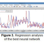 |
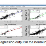
Figure 3: Regression analysis of the best neural network Click here to View figure |
The best results are represented in Tables 4-6, using the MATLAB script. The name of back-propagation algorithm, the variable 74, combined number from Table (4), the number of hidden neurons and also the overall correlation coefficient are represented in these tables.
 |
|
The neural network model could be trained as a two-step process. In the first step, fgf. The specified variables in this case were used in the set 25 at the Table (6), and the new combinations were used by these identified variables.
 |
|
Result and Discussion
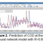
The performance of Tabriz wastewater treatment plant is simulated in this study by a multi-layer neural network and the performance of the treatment plant is evaluated over a period of six months using this advanced model. The sewage treatment plant of Tabriz is modeled in the aspects of a process using the neural network model and by studies on simulating the presumptive developed sewage treatment plant with the single activated sludge process and SSSP software along with the system’s experiences. The obtained simulating results from the developed neural network model is analyzed for the presumptive treatment plant. The highest obtained correlation coefficient in the presumptive sewage treatment plant modeling with the neural network model with SSSP was 0.980. The considered input variables in this study include: Total Dissolved Solids (TDS), raw sewage temperature (T), Total Suspended Solid (TSS), Chemical Oxygen Demand (COD), Biochemical Oxygen Demand (BOD), Mixed Liquor Suspended Solids (MLSS), and Mixed Liquor Volatile Suspended Solids (MLVSS). The concentration of COD is also being considered as the output variable. Using real data from the Tabriz waste treatment plant, the best and most appropriate neural network model is obtained as R equals to 0.898, which indicates a relatively high accuracy considering the error in the input data. Completing the modeling for industrial sewage treatment plants is very difficult, because of nonlinearity of these complex processes and a wide diversity of inflow characteristics such as composition, strength and velocity of flow, and time change and the nature of biological treatment. The obtained results of the present study show that the multilayer designed neural network with eight inputs (MLSS, COD, BOD, TSS, T, pH, TDS, and MLVSS) and also 17 central neurons has done well in predicting the concentration of the output sullage COD and estimating the performance of Tabriz sewage treatment plant regarding the high correlation coefficient and minimum error. The network Trial2, which is selected as the best model, has the highest correlation coefficient (0.8846), minimum RMSE (10.827), and mean absolute error (7.373) at the evaluating stage. The results indicate that this model has further generalizing power than the others. Therefore, it can be said that ANNs could be used for estimating the performance of sewage treatment plants with an acceptable confidence. The ANN modeling technique has desirable properties such as performance, generalization and simplicity, which makes it to be an ideal choice for modeling complex systems like the sewage treatment processes.
References
- Al-Asheh, S., Alfadala, H.E., , Use of artificial neural network black-box modeling for the prediction of wastewater treatment plants performance, Journal of Environmental Management, 83(3), pp. 329–338. (2007)
- Arsiwala , Wastewater treatment, translated by Ahmad Reza Yazdanbakhsh and Kazem Nadaghi, Fardabeh Publishing. (1993)
- Bagheri, Ardebilian, P., Nabi’ei, A., and Bagheri Ardebilian, M., Efficiency evaluation of Zanjan Wastewater Treatment Plant in 2008, twelfth conference on environmental hygiene. (2009)
- Bidstrup, S.M. and Grady Jr., C.P.L. SSSP ^ Simulation of single-sludge processes. J. Water Pollut. Control Fed. 60, 351^361,(1988)
- Caudill, M., neural networks primer: Part I، AI Expert، December، 46-52. (1987)
- Kermani, M., Efficiency boost and economic strengthening of stabilization pond sewage treatment plants, 2nd conference on environmental management and planning. (2012)
- Hamoda, M.F., Al-Gusain, I.A., Hassan, A.H., Integrated wastewater treatment plant performance evaluation using artificial neural network, Water Science and Technology 40ØŒ 55–69. (1999)
- Hecht-Nielsen, R. “Kolmogorov’s Mapping Neural Network Existence Theorem.” Proceedings of the First IEEE International Joint Conference on Neural Networks, New York11–14., (1987): Mehdi Pour
- Nasr, M.S., Moustafa, A.E., and Seif, A.E., , Application of Artificial Neural Network (ANN) for the prediction of EL-AGAMY wastewater treatment plant performance-EGYPT, Alexandria Engineering Journal, 51(1), 37–43. (2012)
- Torghabeh, A., & Shokuhian, M.. Considering the effect of input parameters on prediction accuracy of COD in wastewater of industrial treatment plants using artificial neural networks, 6th national conference on environmental engineering. (2012)
- Pasha Zanoosi, S., Abbasi, M., Aboutorab, H., and Ayati, B., , Evaluating methods for wastewater treatment plants: Gheytarieh Wastewater Treatment Plant case study, Second national conference on water and wastewater with usage approach. (2008)
- Ráduly, B., Gernaey, K.V., Capodaglio, A.G., Mikkelsend, P.S., and Henzed, M., artificial neural networks for rapid WWTP performance evaluation: Methodology and case study, Environmental Modelling & Software, 22(8), 1208–1216. (2007)
- Roger, L.L., Dowla, F.U. “Optimization of Groundwater Remediation using Artificial Neural Networks with Parallel Solute Transport Modelling.” Water Resources Research 30(2) 457-481 (1994):
- Sin, G. “Determination of ASM1 Sensitive Parameters and Simulation Studies for Ankara Wastewater Treatment Plant.” M.S. Thesis, METU (2000)
- ..Soltani Nezhad, A., Afsahi, M., Nakha’di Zadeh, G., & Chalkesh Amiri, M., Evaluating statistics and artificial intelligence models in modeling the wastewater treatment process, National conference on water/wastewater engineering sciences. (2012)
- Torghabeh, A., & Shokuhian, M. Considering performance of industrial treatment plants using artificial neural network model, 6th national conference and specialized exhibition of environmental engineering. (2012)
- Tchobanoglous, G., Burton, F. L. “Wastewater Engineering: Treatment, Disposal and Reuse.” McGraw-Hill Series in Water Resources and Environmental Engineering, (1991).